Fitxategi:2014 militrary expenditures absolute.svg

SVG fitxategi honen PNG aurreikuspenaren tamaina: 512 × 288 pixel. Bestelako bereizmenak: 320 × 180 pixel | 640 × 360 pixel | 1.024 × 576 pixel | 1.280 × 720 pixel | 2.560 × 1.440 pixel.
Bereizmen handikoa (SVG fitxategia, nominaldi 512 × 288 pixel, fitxategiaren tamaina: 1,52 MB)
Fitxategi hau Wikimedia Commonsekoa da. Hango deskribapen orriko informazioa behean duzu. |
Laburpena
| Deskribapena |
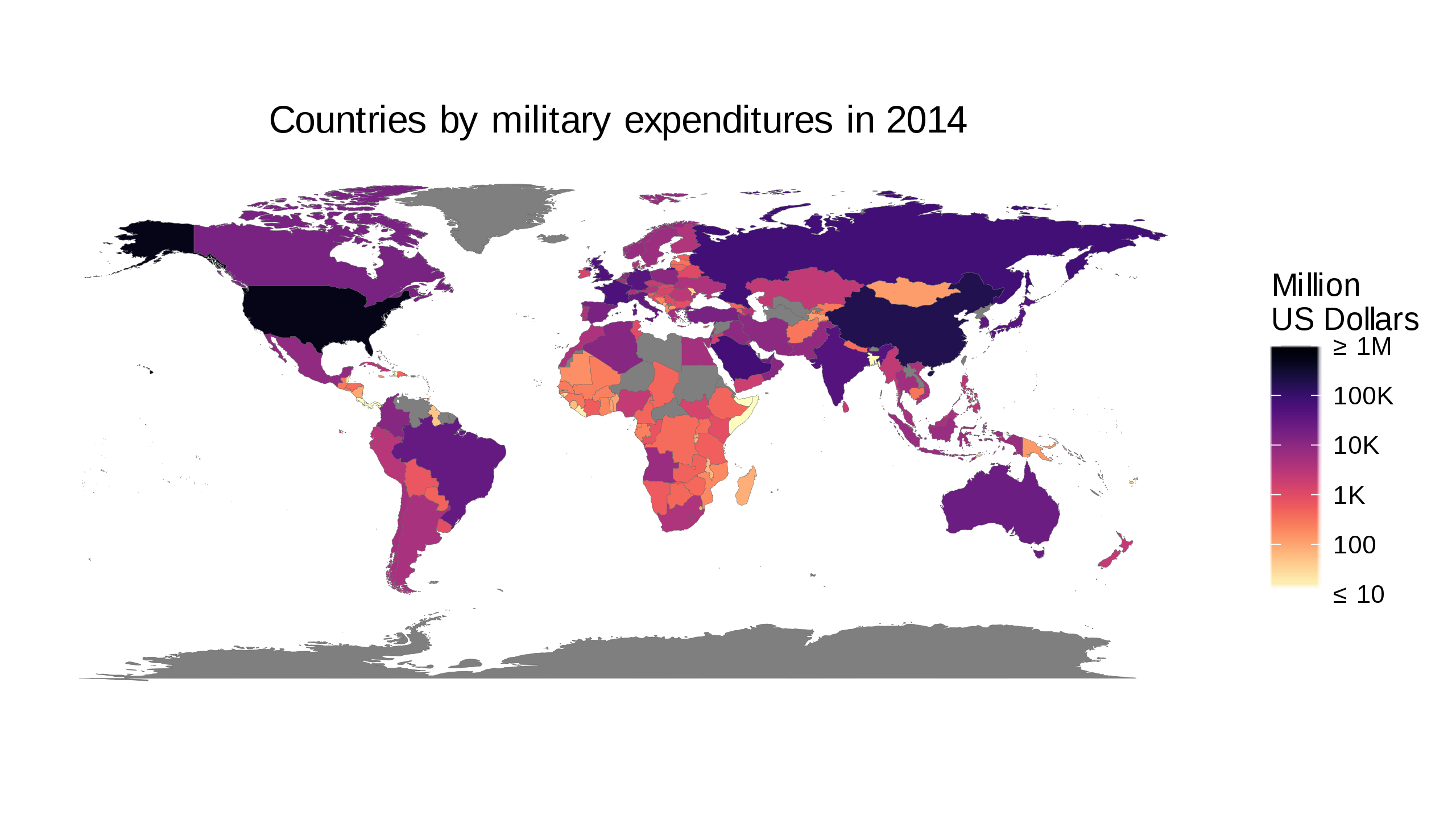
English: Based on the Worldbank data from http://data.worldbank.org/indicator/MS.MIL.XPND.GD.ZS and http://data.worldbank.org/indicator/NY.GDP.MKTP.CD This is a candidate for replacing/augmenting https://commons.wikimedia.org/wiki/File:Countries_by_Military_expenditures_(%25_of_GDP)_in_2014_v2.svg |
| Jatorria | Norberak egina |
| Egilea | Pipping |
_in_2014_v2.svg)
Lizentzia
Nik, lan honen egileak, argitaratzen dut ondorengo lizentzia pean:
This file is licensed under the Creative Commons Attribution-Share Alike 4.0 International license.
- Askea zara:
- partekatzeko – lana kopiatzeko, banatzeko eta bidaltzeko
- birnahasteko – lana moldatzeko
- Ondorengo baldintzen pean:
- eskuduntza – Egiletza behar bezala aitortu behar duzu, lizentzia ikusteko esteka gehitu, eta ea aldaketak egin diren aipatu. Era egokian egin behar duzu hori guztia, baina inola ere ez egileak zure lana edo zure erabilera babesten duela irudikatuz.
- berdin partekatu – Lan honetan oinarrituta edo aldatuta berria eraikitzen baduzu, emaitza lana hau bezalako lizentzia batekin argitaratu behar duzu.
Created with the following piece of code:
library(magrittr)

selectedYear <- 2014

getWorldBankData <- function(indicatorCode, indicatorName) {
    baseName <- paste('API', indicatorCode, 'DS2_en_csv_v2', sep='_')
    ## Download zipfile if necessary
    zipfile <- paste(baseName, 'zip', sep='.')
    if (!file.exists(zipfile)) {
        zipurl <- paste(paste('http://api.worldbank.org/v2/en/indicator',
                              indicatorCode, sep='/'),
                        'downloadformat=csv', sep='?')
        download.file(zipurl, zipfile)
    }
    csvfile <- paste(baseName, 'csv', sep='.')
    ## This produces a warning because of the trailing commas. Safe to ignore.
    readr::read_csv(unz(zipfile, csvfile), skip=4,
                    col_types = list(`Indicator Name` = readr::col_character(),
                                     `Indicator Code` = readr::col_character(),
                                     `Country Name` = readr::col_character(),
                                     `Country Code` = readr::col_character(),
                                     .default = readr::col_double())) %>%
        dplyr::select(-c(`Indicator Name`, `Indicator Code`, `Country Name`))
}

## Obtain and merge World Bank data
worldBankData <-
    dplyr::left_join(
               getWorldBankData('MS.MIL.XPND.GD.ZS') %>%
               tidyr::gather(-`Country Code`, convert=TRUE,
                             key='Year', value=`Military expenditure (% of GDP)`,
                             na.rm = TRUE),
               getWorldBankData('NY.GDP.MKTP.CD') %>%
               tidyr::gather(-`Country Code`, convert=TRUE,
                             key='Year', value=`GDP (current US$)`,
                             na.rm = TRUE)) %>%
    dplyr::mutate(`Military expenditure (current $US)` =
                      `Military expenditure (% of GDP)`*`GDP (current US$)`/100) %>%
    dplyr::filter(Year == selectedYear) %>%
    dplyr::mutate(Year = NULL)

## Plotting: Obtain Geographic data
mapData <- tibble::as.tibble(ggplot2::map_data("world")) %>%
    dplyr::mutate(`Country Code` =
                      countrycode::countrycode(region, "country.name", "iso3c"),
                  ## This produces a warning but I do not see how we could do better
                  ## since we started with fuzzy names.
                  region = NULL, subregion = NULL)

combinedData <- dplyr::left_join(mapData, worldBankData)

## The default out-of-bounds function `censor` replaces values outside
## the range with NA. Since we have properly labelled the legend, we can
## project them onto the boundary instead
clamp <- function(x, range = c(0, 1)) {
    lower <- range[1]
    upper <- range[2]
    ifelse(x > lower, ifelse(x < upper, x, upper), lower)
}

ggplot2::ggplot(data = combinedData, ggplot2::aes(long,lat)) +
    ggplot2::geom_polygon(ggplot2::aes(group = group,
                                       fill  = `Military expenditure (current $US)`),
                          color = '#606060', lwd=0.05) +
    ggplot2::scale_fill_gradientn(colours= rev(viridis::magma(256, alpha = 0.5)),
                                  name   = "Million\nUS Dollars",
                                  trans  = "log",
                                  oob    = clamp,
                                  breaks = c(1e7,1e8,1e9,1e10,1e11,1e12),
                                  labels = c('\u2264 10', '100', '1K',
                                             '10K', '100K', '\u2265 1M'),
                                  limits = c(1e7,1e12)) +
    ggplot2::coord_fixed() +
    ggplot2::theme_bw() +
    ggplot2::theme(plot.title = ggplot2::element_text(hjust = 0.5),
          axis.title = ggplot2::element_blank(),
          axis.text = ggplot2::element_blank(),
          axis.ticks = ggplot2::element_blank(),
          panel.grid.major = ggplot2::element_blank(),
          panel.grid.minor = ggplot2::element_blank(),
          panel.border = ggplot2::element_blank(),
          panel.background = ggplot2::element_blank()) +
    ggplot2::labs(title = paste("Countries by military expenditures in",
                                selectedYear))

ggplot2::ggsave(paste(selectedYear, 'militrary_expenditures_absolute.svg', sep='_'),
                height=100, units='mm')
Fitxategiaren historia
Data/orduan klik egin fitxategiak orduan zuen itxura ikusteko.
| Data/Ordua | Iruditxoa | Neurriak | Erabiltzailea | Iruzkina | |
|---|---|---|---|---|---|
| oraingoa | 16:30, 20 maiatza 2017 | | 512 × 288 (1,52 MB) | Pipping | redo with dplyr |
| 14:12, 13 maiatza 2017 |  | 512 × 256 (1,51 MB) | Pipping | Handle truncation of the data range better: We distinguish between 0 and no data, but any existing datum below 10M USD is coloured the same way and all data above 1T USD are coloured the same way. The legend makes this clear. | |
| 10:55, 13 maiatza 2017 |  | 512 × 256 (1,51 MB) | Pipping | Completely redone. The former was in local currency (so that comparisons from country to country made absolutely no sense). Now everything is in current US dollars. | |
| 00:32, 12 maiatza 2017 |  | 512 × 256 (1,5 MB) | Pipping | Fixed min/max value for colors that kept anything below 1,000,000,000 US dollars from having a colour (now: Anything above 1,000,000 US dollars has a colour). | |
| 23:30, 11 maiatza 2017 |  | 512 × 256 (1,51 MB) | Pipping | {{Information |Description ={{en|1=English: Based on the Worldbank data from http://data.worldbank.org/indicator/MS.MIL.XPND.CN This is a candidate for replacing/augmenting https://commons.wikimedia.org/wiki/File:Countries_by_Military_expenditures_(... |
Irudira dakarten loturak
Hurrengo orrialdeek dute fitxategi honetarako lotura:
Fitxategiaren erabilera orokorra
Hurrengo beste wikiek fitxategi hau darabilte:
- bg.wikipedia.org proiektuan duen erabilera
- ca.wikipedia.org proiektuan duen erabilera
- en.wikipedia.org proiektuan duen erabilera
- sr.wikipedia.org proiektuan duen erabilera
- th.wikipedia.org proiektuan duen erabilera
- uk.wikipedia.org proiektuan duen erabilera